This function processes tracking data for a specific tag and generates a
visualization using ggplot2. It allows customization of colors, point
sizes, and track styles, and supports various display options such as
datetime, nbs (number of base stations / receivers), standard deviation,
speed_in and gap. The function can either return the plot or save it as an
png file.
Usage
atl_check_tag(
  data,
  buffer = 1000,
  asp = "16:9",
  option = "datetime",
  scale_option = "A",
  scale_direction = -1,
  scale_trans = "identity",
  scale_max = NULL,
  first_n = NULL,
  last_n = NULL,
  highlight_first = FALSE,
  highlight_last = FALSE,
  highlight_outliers = FALSE,
  point_size = 0.5,
  point_alpha = 1,
  path_linewidth = 0.5,
  path_alpha = 0.1,
  element_text_size = 11,
  water_fill = "#D7E7FF",
  water_colour = "grey80",
  land_fill = "#faf5ef",
  land_colour = "grey80",
  mudflat_colour = "#faf5ef",
  mudflat_fill = "#faf5ef",
  mudflat_alpha = 0.6,
  filename = NULL,
  png_width = 3840,
  png_height = 2160
)
Arguments
- data
A
data.tablecontaining tracking data. Must include the columns:"tag","x","y","time", and"datetime".- buffer
Numeric. The buffer size in meters around the data points in the plot (default: 1000).
- asp
The aspect ratio of the plot (default:
"16:9").- option
Determines the color mapping variable. Options are:
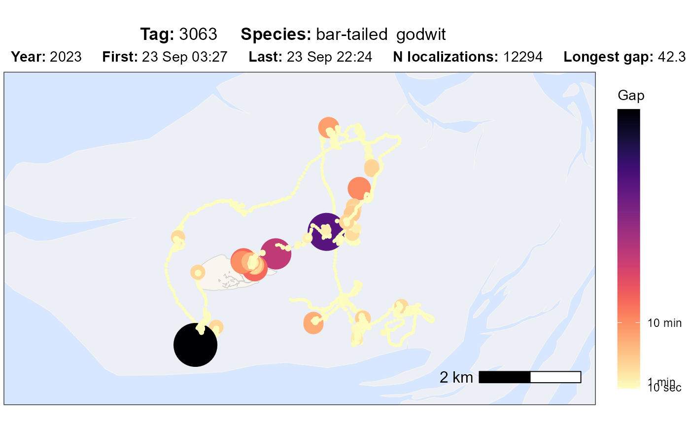
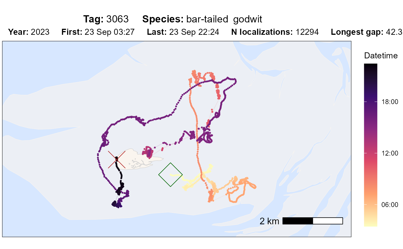
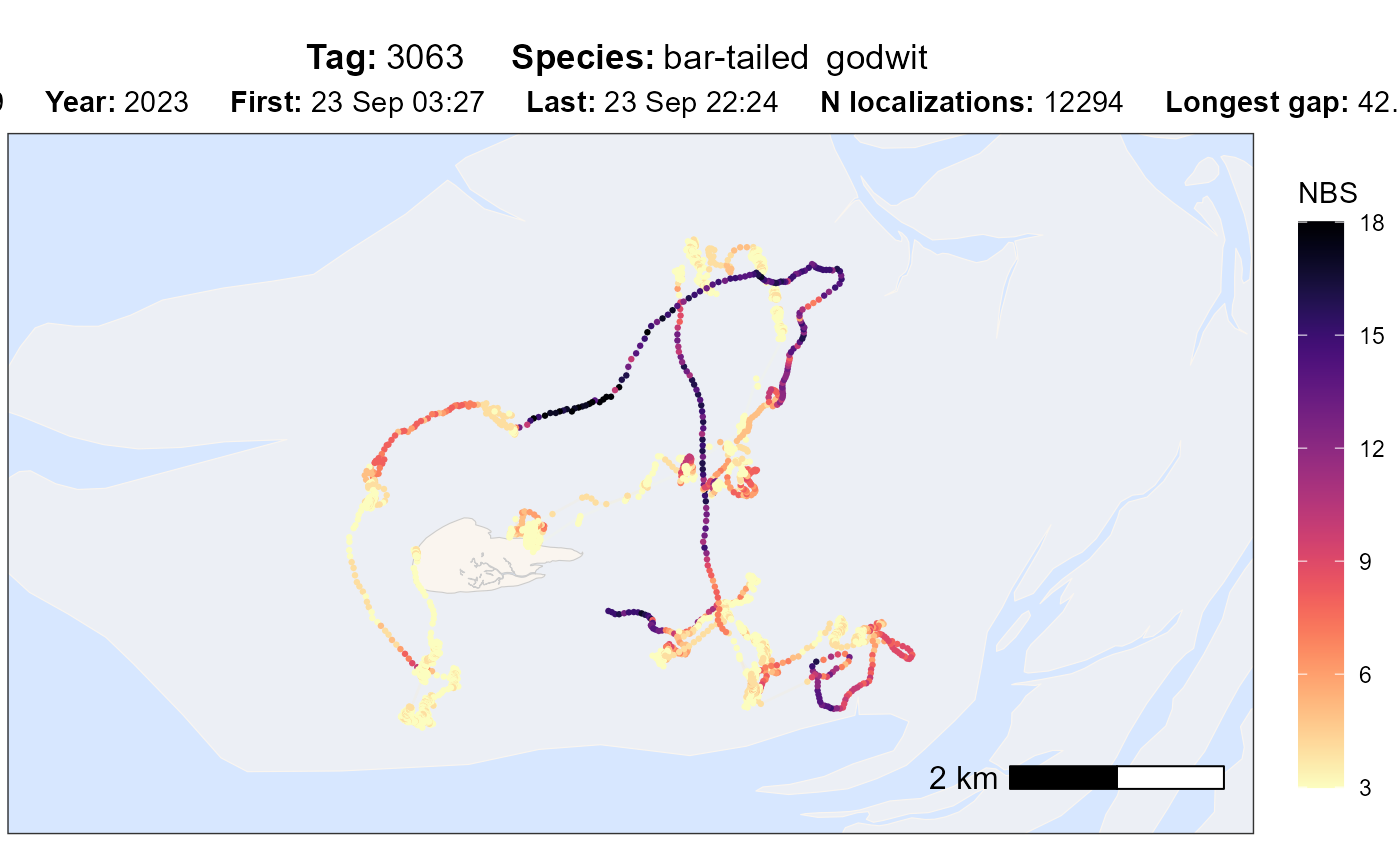
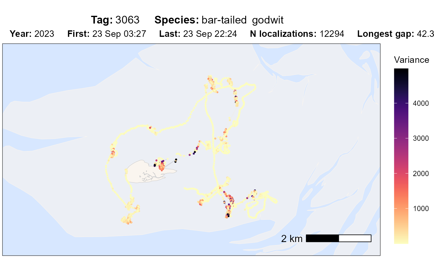
"datetime": Datetime along the track"nbs": Number of receiver (base) stations that contributed to the localization"var": Error as maximal variance of varx and vary"speed_in": Speed in m/s"gap": Gaps coloured by time and as point size
- scale_option
Character. The color scheme option from
viridis(default:"A"). See https://search.r-project.org/CRAN/refmans/viridisLite/html/viridis.html for all options (A-H).- scale_direction
Numeric. Direction of the color scale (-1 reverses, default: -1).
- scale_trans
Transformation of the scale. Default is "identity", (no transformation), could be e.g. "log", "log10" or "sqrt". See scale_*_trans() for all options.
- scale_max
If set, determines the max value of the scale for options: nbs (numeric), var (numberic), speed_in (numeric m/s), gap (numeric in seconds). Everything above the max value will get the max color.
- first_n
Numeric (or NULL). If provided, only the first
nlocations are shown.- last_n
Numeric (or NULL). If provided, only the last
nlocations are shown.- highlight_first
Logical. If
TRUE, highlights the first point in the track (default:FALSE).- highlight_last
Logical. If
TRUE, highlights the last point in the track (default:FALSE).- highlight_outliers
Logical. If
TRUE, highlights all points that are flagged as outliers (needs preassigned column with outlier TRUE or FALSE) track (default:FALSE).- point_size
The size of the data points (default: 0.5).
- point_alpha
Numeric. Transparency of the data points (default: 1).
- path_linewidth
Numeric. The width of the connecting track lines (default: 0.5).
- path_alpha
Transparency of the track lines (default: 0.1).
- element_text_size
Adjust size of the text.
- water_fill
Water fill (default "#D7E7FF")
- water_colour
Water coulour (default "grey80")
- land_fill
Land fill (default "#faf5ef")
- land_colour
Land colour (default "grey80")
- mudflat_colour
Mudflat colour (default "#faf5ef")
- mudflat_fill
Mudflat fill (default "#faf5ef")
- mudflat_alpha
Mudflat alpha (default 0.6)
- filename
Character (or NULL). If provided, the plot is saved as a
.pngfile to this path and with this name; otherwise, the function returns the plot.- png_width
Width of saved PNG (default: 3840).
- png_height
Height of saved PNG (default: 2160).
Value
A ggplot2 object with the specified option and adjustments. If
filename is provided, the plot is saved as a .png file instead of
being returned.
Examples
# packages
library(tools4watlas)
# path to csv with filtered data
data_path <- system.file(
"extdata", "watlas_data_filtered.csv",
package = "tools4watlas"
)
# load data
data <- fread(data_path, yaml = TRUE)
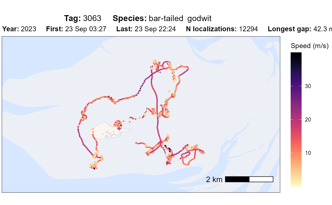
# subset bar-tailed godwit
data <- data[species == "bar-tailed godwit"]
# plot different options
atl_check_tag(
data,
option = "datetime",
highlight_first = TRUE, highlight_last = TRUE
)
 atl_check_tag(data, option = "nbs")
 atl_check_tag(data, option = "var")
 atl_check_tag(data, option = "speed_in")
 atl_check_tag(data, option = "gap")