Filters out positions lying inside or outside an area.
The area can be defined in two ways, either by its x- and y-coordinate
ranges, or by an sf-POLYGON object.
MULTIPOLYGON objects are supported by the internal function
atl_within_polygon.
Usage
atl_filter_bounds(
  data,
  x = "x",
  y = "y",
  x_range = NA,
  y_range = NA,
  sf_polygon = NULL,
  remove_inside = TRUE
)
Arguments
- data
A
data.tableor extension which contains x- and y-coordinates.- x
The x coordinate column.
- y
The y coordinate column.
- x_range
The range of x coordinates.
- y_range
The range of y coordinates.
- sf_polygon
sfc_POLYGONobject which must have a defined CRS. The polygon CRS is assumed to be appropriate for the positions as well, and is assigned to the coordinates when determining the intersection.- remove_inside
Whether to remove points from within the range. Setting
negate = TRUEremoves positions within the bounding box specified by the x- and y-ranges.
Examples
# packages
library(tools4watlas)
library(sf)
library(ggplot2)
# load example data
data <- data_example
# create basemap
bm <- atl_create_bm(data, buffer = 800)
# create a bounding box to filter data
griend_east <- st_sfc(st_point(c(5.275, 53.2523)), crs = st_crs(4326)) |>
st_transform(crs = st_crs(32631))
# define bbox to crop data
bbox_crop <- atl_bbox(griend_east, asp = "16:9", buffer = 2000)
bbox_sf <- st_as_sfc(bbox_crop) # just for plotting as sf object
# geom_sf overwrites coordinate system, so we need to set the limits again
bbox <- atl_bbox(data, buffer = 800)
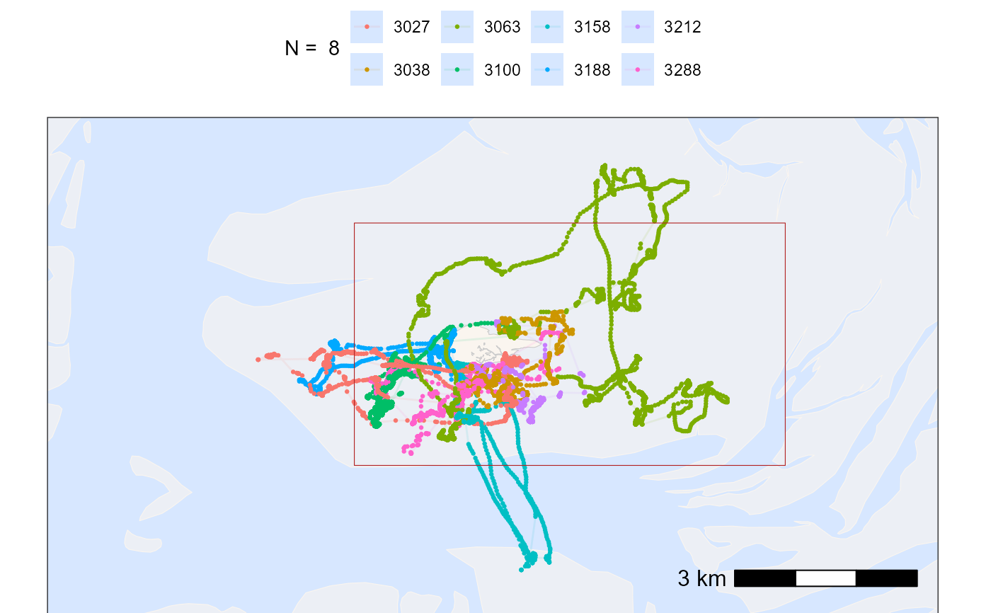
# plot points and tracks with standard ggplot colours
bm +
geom_path(
data = data, aes(x, y, colour = tag),
linewidth = 0.5, alpha = 0.1, show.legend = TRUE
) +
geom_point(
data = data, aes(x, y, colour = tag),
size = 0.5, alpha = 1, show.legend = TRUE
) +
geom_sf(data = bbox_sf, color = "firebrick", fill = NA) +
scale_color_discrete(name = paste("N = ", length(unique(data$tag)))) +
theme(legend.position = "top") +
# set extend again (overwritten by geom_sf)
coord_sf(
xlim = c(bbox["xmin"], bbox["xmax"]),
ylim = c(bbox["ymin"], bbox["ymax"]), expand = FALSE
)
#> Coordinate system already present.
#> ℹ Adding new coordinate system, which will replace the existing one.
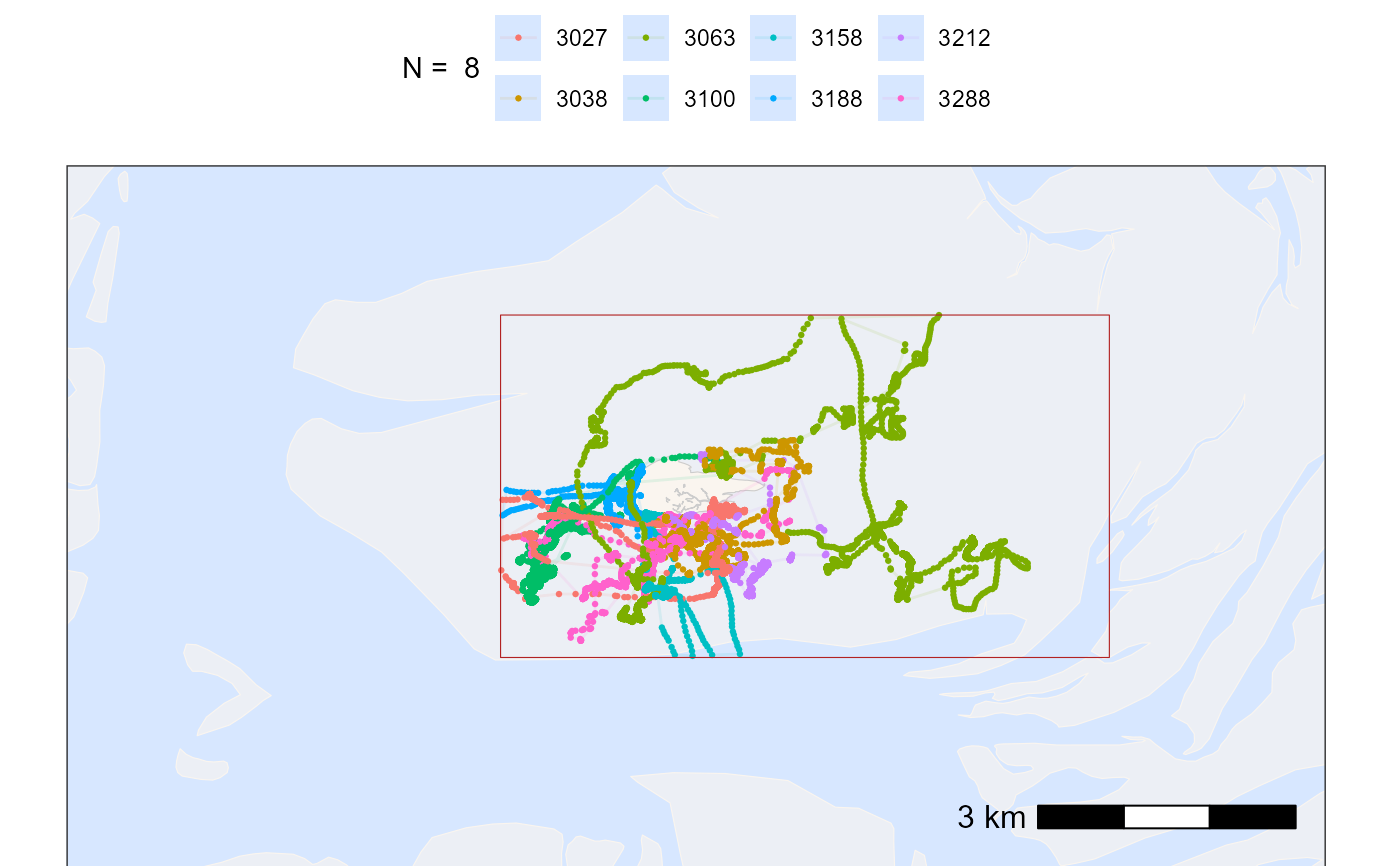
 # filter data with bounding box
# note: when filtering with a rectangle bounding box
# and large datasets, using th range is faster than sf_polygon
data_filtered <- atl_filter_bounds(
data = data,
x = "x",
y = "y",
x_range = c(bbox_crop["xmin"], bbox_crop["xmax"]),
y_range = c(bbox_crop["ymin"], bbox_crop["ymax"]),
remove_inside = FALSE
)
# plot cropped data
bm +
geom_path(
data = data_filtered, aes(x, y, colour = tag),
linewidth = 0.5, alpha = 0.1, show.legend = TRUE
) +
geom_point(
data = data_filtered, aes(x, y, colour = tag),
size = 0.5, alpha = 1, show.legend = TRUE
) +
geom_sf(data = bbox_sf, color = "firebrick", fill = NA) +
scale_color_discrete(name = paste("N = ", length(unique(data$tag)))) +
theme(legend.position = "top") +
# set extend again (overwritten by geom_sf)
coord_sf(
xlim = c(bbox["xmin"], bbox["xmax"]),
ylim = c(bbox["ymin"], bbox["ymax"]), expand = FALSE
)
#> Coordinate system already present.
#> ℹ Adding new coordinate system, which will replace the existing one.
# filter data with bounding box
# note: when filtering with a rectangle bounding box
# and large datasets, using th range is faster than sf_polygon
data_filtered <- atl_filter_bounds(
data = data,
x = "x",
y = "y",
x_range = c(bbox_crop["xmin"], bbox_crop["xmax"]),
y_range = c(bbox_crop["ymin"], bbox_crop["ymax"]),
remove_inside = FALSE
)
# plot cropped data
bm +
geom_path(
data = data_filtered, aes(x, y, colour = tag),
linewidth = 0.5, alpha = 0.1, show.legend = TRUE
) +
geom_point(
data = data_filtered, aes(x, y, colour = tag),
size = 0.5, alpha = 1, show.legend = TRUE
) +
geom_sf(data = bbox_sf, color = "firebrick", fill = NA) +
scale_color_discrete(name = paste("N = ", length(unique(data$tag)))) +
theme(legend.position = "top") +
# set extend again (overwritten by geom_sf)
coord_sf(
xlim = c(bbox["xmin"], bbox["xmax"]),
ylim = c(bbox["ymin"], bbox["ymax"]), expand = FALSE
)
#> Coordinate system already present.
#> ℹ Adding new coordinate system, which will replace the existing one.