Plot data in base R

Johannes Krietsch

Load packages

This article shows how to plot WATLAS data with base R

# packages
library(tools4watlas)

Base R plotting

Plot with simple base map

The plotting region can be extended by specifiying buffer (in meters), and the scale of the scalebar (in kilometers) can be adjusted. To inspect the localizations, color_by can be specified to colour the localizations by time since first localization in plot (“time”), standard deviation of the x- and y-coordinate (“sd”), or the number of base stations used for calculating the localization (“nbs”). By specifiying the full path and file name (with extension) in fullname, it is possible to save the plot as a .png. If necesarry, the legend can also be located elsewhere on the plot with Legend.

# load example data
data <- data_example[tag == data_example[1, tag]]

# transform to sf
d_sf <- atl_as_sf(data, additional_cols = names(data))

# plot the tracking data with a simple background
atl_plot_tag(
  data = d_sf, tag = NULL, fullname = NULL, buffer = 1,
  color_by = "time"
)

## [1] "Ensure that data has the UTM 31N coordinate reference system."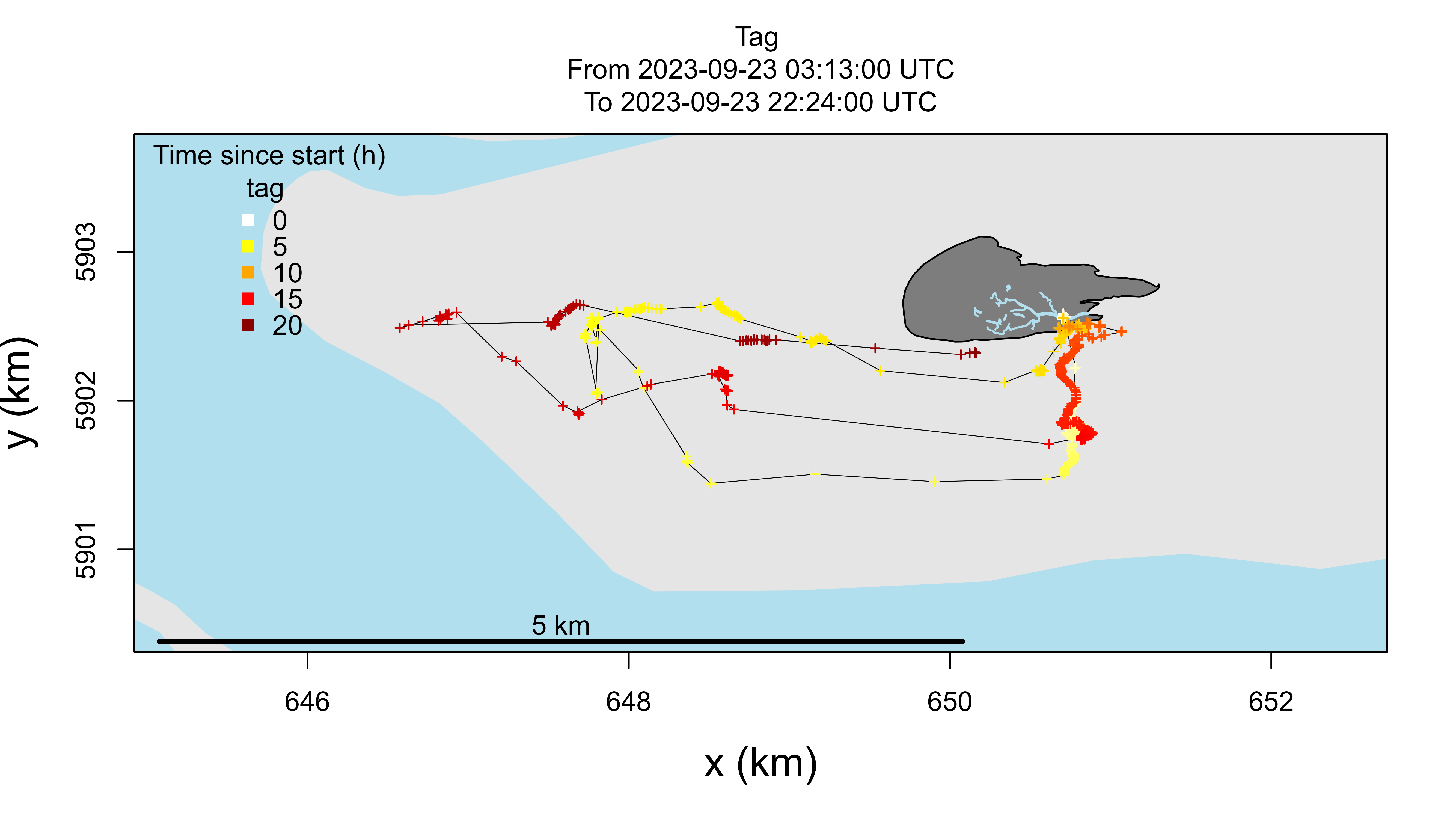

Base R map

# note: function opens device and therefore the plot is not shown in markdown

Plot with OpenStreetMap

With the function atl_plot_tag_osm() it is possible to plot the track on a satellite image with the library OpenStreetMap. The region of the the satellite image can be extended by specifying a buffer (in meters) in the function atl_bbox The other options are similar to atl_plot_tag (see earlier).

library(OpenStreetMap)
library(sf)

# load example data
data <- data_example[tag == data_example[1, tag]]

# make data spatial and transform projection to WGS 84 (used in osm)
d_sf <- atl_as_sf(data, additional_cols = names(data))
d_sf <- sf::st_transform(d_sf, crs = sf::st_crs(4326))

# get bounding box
bbox <- atl_bbox(d_sf, buffer = 500)

# extract openstreetmap
# other 'type' options are "osm", "maptoolkit-topo", "bing", "stamen-toner",
# "stamen-watercolor", "esri", "esri-topo", "nps", "apple-iphoto", "skobbler";
map <- OpenStreetMap::openmap(c(bbox["ymax"], bbox["xmin"]),
  c(bbox["ymin"], bbox["xmax"]),
  type = "osm", mergeTiles = TRUE
)

# plot the tracking data on the satellite image
atl_plot_tag_osm(
  data = d_sf, tag = NULL, mapID = map, color_by = "time",
  fullname = NULL, scalebar = 3
)

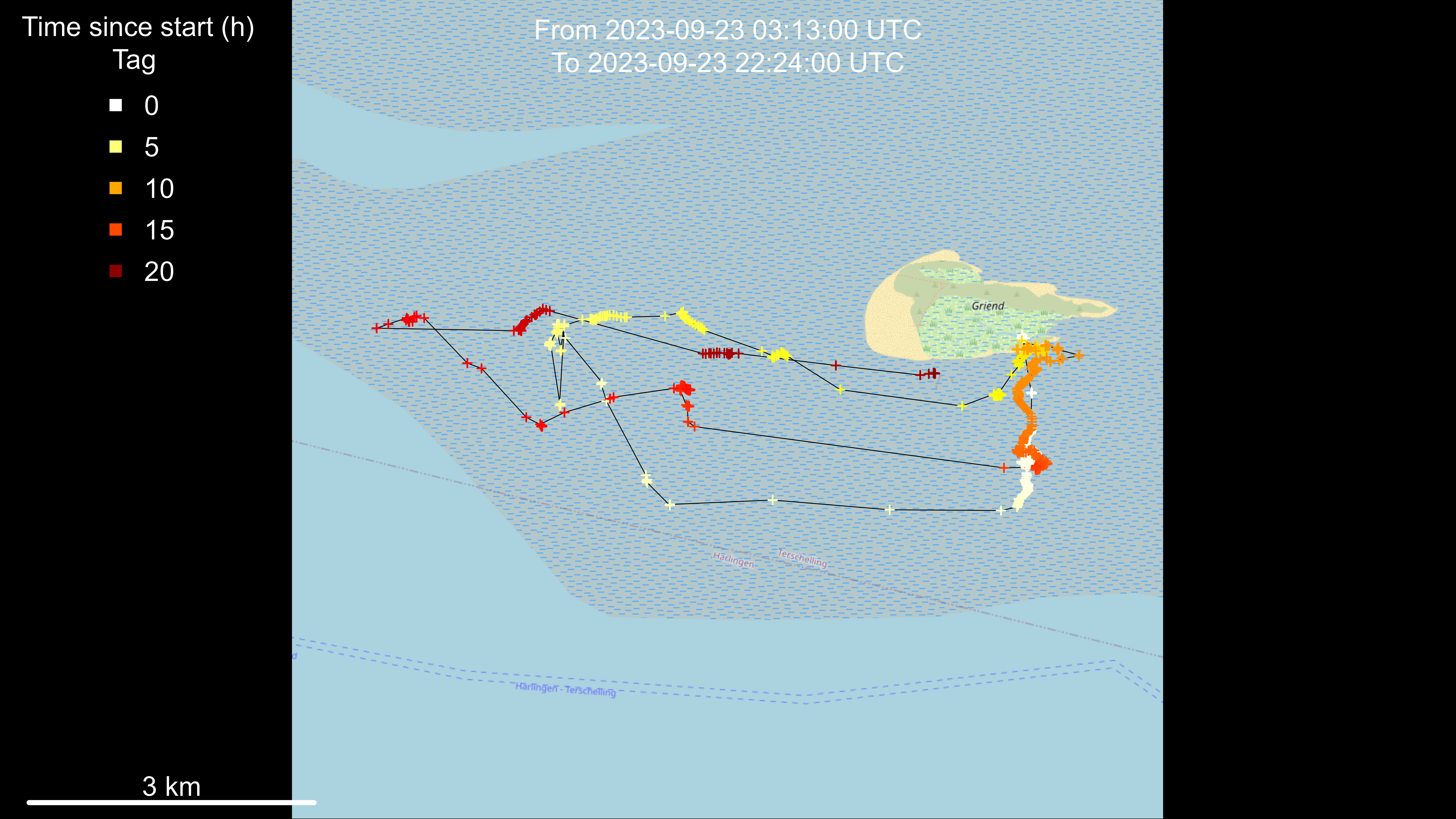
Base R map with satellite image